Performance Analysis Tools
Introduction to Performance Anlysis Tools
BSC Machines provide an amount of in-house developed performance analysis tools, so developers/researchers can trace and examine their programs to identify and solve issues and improve their efficiency.
Extrae
Remember to check their documentation for more information and other learning material.
Extrae is a dynamic instrumentation package to trace programs compiled and run with the shared memory model (like OpenMP and pthreads), the message passing �MPI� programming model or both programming models (different MPI processes using OpenMP or pthreads within each MPI process). Extrae generates trace files that can be later visualized with Paraver.
Instrumentation Mechanism
Extrae has different methods to intercept library calls to instrument them, but in this page we will only cover the LD_PRELOAD method. LD_PRELOAD is an environment variable that will tell the system to load an specific library on top of all the others. As Extrae also has the functions (of MPI, OpenMP, and supported libraries) defined for the instrumentation, when we preload the Extrae library we will be instrumenting the application.
Extrae is compiled into diferent libraries that support different sets of libraries. For example we have the libmpitrace.so that intercepts the MPI calls to instrument them. But for OpenMP we should use another library (libomptrace.so). If you want more information on how to enable support for more libraries visit the documentation here.
When our application is implemented in Fortran we have to use a specific library that is the same as the library for C but appending an f at the end of the name. For example the library for Fortran applications with MPI would be libmpitracef.so.
To set the LD_PRELOAD variable and run the application we usually use a loading script. The developers usually call that script trace.sh, an example of this file is:
#!/bin/bash
source /apps/BSCTOOLS/extrae/4.0.1/impi_2017_4/etc/extrae.sh
export EXTRAE_CONFIG_FILE=../extrae.xml
export LD_PRELOAD=${EXTRAE_HOME}/lib/libmpitrace.so
## Run the desired program
$*
Then to run (in this case an MPI application) we could run the command as this:
mpirun -n 48 ./trace.sh ./application
Configuration
Extrae has instrumentation implemented for several libraries and different features that can be independently activated/deactivate. To do so Extrae requires a configuration file in XML format (usually extrae.xml). To tell Extrae where this file can be found we use an environment variable �EXTRAE_CONFIG_FILE�, usually set in the ld-preload script.
You can find in extrae_explained.xml (under $EXTRAE_HOME/share/example once the module is loaded) an example of this file with all the options explained by the developers, in the examples folder.
When we want to trace an MPI application as well as using a MPI enabled Extrae library (the more basic is libmpitrace.so) we have to enable the MPI tracing in the configuration.
Using the enabled option of the mpi field, we can also activate the counters for MPI (this will tell extrae to capture the counters for all the MPI processes). The piece of configuration file that would activate this features is the following:
<!-- Configuration of some MPI dependant values -->
<mpi enabled="yes">
<!-- Gather counters in the MPI routines? -->
<counters enabled="yes" />
<!-- Capture all MPI_Comm_* calls? -->
<comm-calls enabled="yes" />
</mpi>
When our application uses OpenMP as well as using an OpenMP enabled Extrae library (as always, in this case the more basic is libopmtrace.so) we have to enable it in the config file. And following you can find an example of what the OpenMP configuration ought to be on an OpenMP tracing run.
<!-- Configuration of some OpenMP dependant values -->
<openmp enabled="yes" ompt="no">
<!-- If the library instruments OpenMP, shall we gather info about locks? Obtaining such information can make the final trace quite large. -->
<locks enabled="no" />
<!-- Gather info about taskloops? -->
<taskloop enabled="no" />
<!-- Gather counters in the OpenMP routines? -->
<counters enabled="yes" />
</openmp>
In the case of having an MPI+�OpenMP application we should use the Extrae library that has both MPI and OpenMP enabled (libompitrace.so). And we should activate both options in the configuration file.
To activate the counters we enable the counters, cpu, and set, and we define the PAPI counters that we want to use inside the set option. As follows in the example.
<!-- Configure which software/hardware counters must be collected -->
<counters enabled="yes">
<cpu enabled="yes" starting-set-distribution="1">
<set enabled="yes" domain="all" changeat-time="0">
PAPI_TOT_INS,PAPI_TOT_CYC
</set>
</cpu>
</counters>
To see which counters are available, you can execute the command papi_avail. It is normal to see a lot of unavailable counters in MN, you need to have activated the constraint perfparanoid in either your reservation or your job, then that counters will become available.
Paraver
This is the tool that we use to visualize the time stamped data generated by Extrae. This tool will read the file and create diferent visual representations for the diferent events in the trace.
Starting Paraver
To use Paraver first you have to install it, or if you are using one of the BSC HPC machines you can use the already installed one with an ssh X session.
To install Paraver on your system, you can either compiled yourself or use a compiled version. You can download the source code or the binary from this website.
I you want to run Paraver on an HPC machine you will need to first load the module by running
module load paraver
First of all you have to load the trace or traces you want to use. You can do it directly from the terminal by running wxparaver trace1.prv trace2.prv, or you can also start Paraver without any trace loaded by running the command wxparaver without any option. And then opening a trace via the top bar options: File -> Load Trace... (or using the keyboard shortcut, Ctrl+O).
Views
A Paraver view displays information about specific events in traces, this information is displayed in a grid, where each row represents on "Object" and each column an instance in time.
An "Object" can be a process or can be a thread, or a thread of a process, depending on the application. Then some information about the events can be painted. Usually we paint the "ast Event value" and this is the one that will be covered in this tutorial. This information can painted as different things. The two most used are code color, where each color represents some discrete value.
Or on the other hand in color gradients, where a gradient of colors (usually from green to blue) represent a set of continuous values.
Some configurations are already pre-made and can be accessed via the "Hints" menu in the top bar. You can also find more configurations using the "Load Configuration..." option in the "File" menu in the top bar.
An example of a view is:
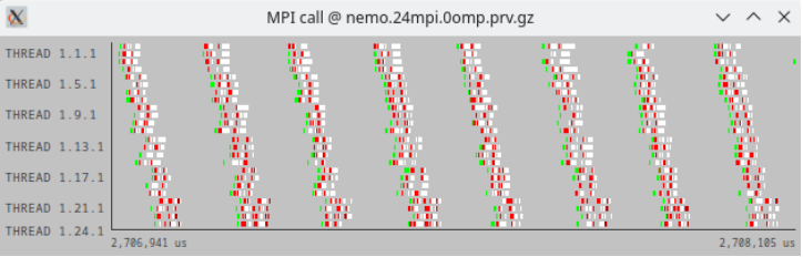
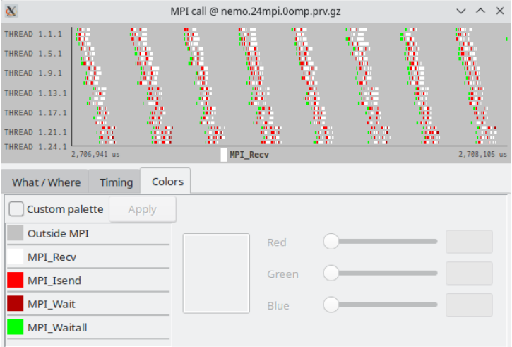
With a right click on top of the trace and selecting the "Info Panel" you can visualize the meaning of each color (in the Color tab), as shown below:
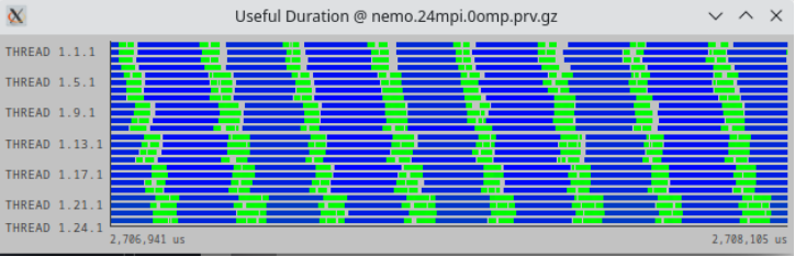
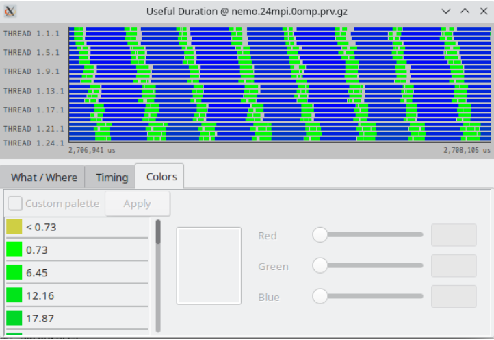
You can also paint the traces as Color gradients, in this case below you can observe the useful duration. In this case the color green represents low values of micro seconds, and blue ones represent higher ones.
You can as well in the same way visualize the color scale using the "Info Panel" as shown below.
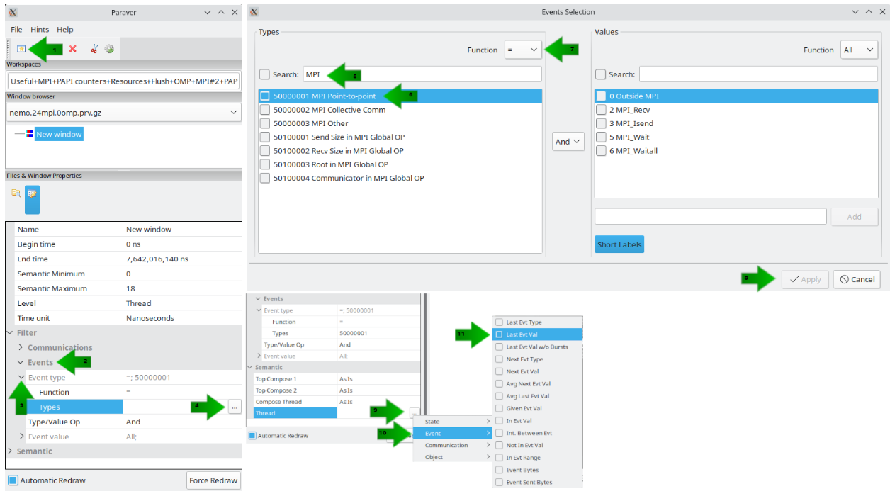
To create your own view you can follow the steps indicated by the arrows. And to create views for events other than MPI Point to Point calls you can tweak steps 5 and 6.
Flags
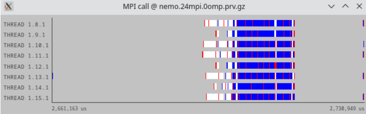
Usually you will see traces with a lot of events very near to each other, so that it looks like only one big event. Just like in the image below.
Before taking conclusions and assuming that this is only a hand full of blue events, if we enable the Flags, we will be able to see each event's beginning and end. To do so we use the right-click menu, and in the "View" option enable the "Flags".
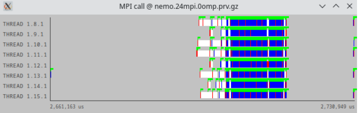
Once the flags are activated you can see how a lot of green appears, meaning that there are many events. If we zoom in we can observe the different events.
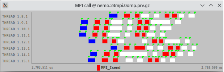
Once we start zooming we can see how the density of the flags start to decrease, up to the point where we can see each one separately.
Communication lines
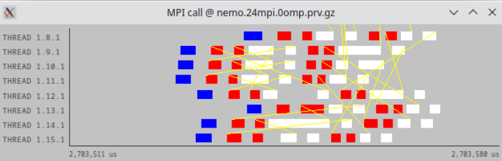
Usually, with applications that have communication, it is useful to see for each communication call to whom it is communicating. To do so Paraver has the "Communication Lines". And to activate them you need to open the "right click" menu and in the "View" option select "Communication Lines". Then you will be able to observe the communication as in the image below
Draw mode
Sometimes when you have a trace with a lot of events, more than one event should be painted in the same pixel, this is a problem since every pixel can only paint one colour.
To solve that Paraver introduces the draw mode. The draw mode is a function to select the colour of the pixel taking into account all the events that should have to be painted. An example of draw mode is the maximum, if you select this function whenever you have several events the one with a higher value will be the one that makes it to the pixel.
TALP
TALP (Tracking Application Life Performance) is a portable, extensible, lightweight, and scalable tool for parallel performance measurement. TALP implements the well defined and established POP metrics and offers an API to consult them during the execution.
The efficiency metrics reported by TALP allow HPC users to evaluate the parallel efficiency of their executions, both post-mortem and at runtime.
Metrics
TALP measures how efficient is your execution in terms of Parallel efficiency. This Parallel efficiency indicates the amount of time that is being lost due to the parallelization of the code. Or, what is the same, the ratio between the time that is being used for useful computation and the total consumed CPU time.
As we said, the Parallel efficiency PE can be computed as the product of the Load balance LB and Communication efficiency.
The Load balance measures the efficiency loss due to different loads (useful computation) for each process. And the Communication efficiency the time spent in communication that is not due to Load imbalance. Communication Efficiency is the product of the Transfer and the Serialization but as these two metrics cannot be computed online we will not enter into their details
Usage
Its usage it is easy and integrated in MareNostrum4 and UserPortal so it becames transparent to the user. With the aim to expand it to the rest of BSC Clusters.
The activation of TALP for your MPI code is as easy as:
module load talp
After that, the mpirun command will invoke a wrapper for everything to be set up to use TALP to trace the code. You just have to execute your mpirun program as usual, p.e:
mpirun ./application
The same can be done with srun:
srun ./application
If the execution finishes successfully, your job report in UserPortal will include a box with the reported metrics for it.
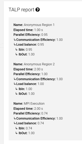
As seen in the screenshot, the feature also supports the report of various regions when the API is used. It is important to note that two regions cannot have the same name.
Educational resources
To a better understanding of the POP Metrics and to learn about Performance Analysis, you can visit these webpages you might find useful: